
House Price Prediction
This is the first practice for machine learning and for Kaggle competition: House Prices: Advanced Regression Techniques. Using Ridge, Lasso, LGBM, XGB, Stacking CV Regressor, and etc, to reach Score(mean absolute error): 11977.59807; 13th place out of 19,465 teams (0.06%) For more information, please see my project directly or visit my Github Repository.
![]()
version 1: Simple Prediction(with ridge regression, random forest, bagging, XGBoost) View PDF
version 2: Score(root mean squared logarithmic error): 0.10643; Rank: top 2%. score: 0.10643;
version3: Score(mean absolute error): 11977.59807; Rank: 13 out of 19,465 teams(0.06%)
House Price Prediction — version 2
Charles Zhang Jan 19 2020
Introduction

This is my second version House Price Prediction Model for the Kaggle Competition. In this version, I improve methods for processing missing value more accurately, use Ridge, Lasso, LGBM, XGB, and Stacking CV Regressor to build machie learning models, and add blended models. Since some contents are repeated, I will just breifly describe the dataset at the beginning.
# This Python 3 environment comes with many helpful analytics libraries installed
# It is defined by the kaggle/python docker image: https://github.com/kaggle/docker-python
# For example, here's several helpful packages to load in

import numpy as np # linear algebra
import pandas as pd # data processing, CSV file I/O (e.g. pd.read_csv)

# Input data files are available in the "../input/" directory.
# For example, running this (by clicking run or pressing Shift+Enter) will list the files in the input directory
import matplotlib.gridspec as gridspec
from datetime import datetime
from scipy.stats import skew  # for some statistics
from scipy.special import boxcox1p
from scipy.stats import boxcox_normmax
from sklearn.linear_model import ElasticNetCV, LassoCV, RidgeCV
from sklearn.ensemble import GradientBoostingRegressor
from sklearn.svm import SVR
from sklearn.pipeline import make_pipeline
from sklearn.preprocessing import RobustScaler
from sklearn.model_selection import KFold, cross_val_score
from sklearn.metrics import mean_squared_error
from mlxtend.regressor import StackingCVRegressor
from xgboost import XGBRegressor
from lightgbm import LGBMRegressor
import matplotlib.pyplot as plt
import scipy.stats as stats
import sklearn.linear_model as linear_model
import matplotlib.style as style
import seaborn as sns
from sklearn.manifold import TSNE
from sklearn.cluster import KMeans
from sklearn.decomposition import PCA
from sklearn.preprocessing import StandardScaler


import warnings
warnings.filterwarnings('ignore')

# Any results you write to the current directory are saved as output.
A Glimpse of the datasets.
train = pd.read_csv("../input/house-prices-advanced-regression-techniques/train.csv")
test = pd.read_csv("../input/house-prices-advanced-regression-techniques/test.csv")
# gives us statistical info about the numerical variables.
train.describe().T
| count | mean | std | min | 25% | 50% | 75% | max | |
|---|---|---|---|---|---|---|---|---|
| Id | 1460.0 | 730.500000 | 421.610009 | 1.0 | 365.75 | 730.5 | 1095.25 | 1460.0 |
| MSSubClass | 1460.0 | 56.897260 | 42.300571 | 20.0 | 20.00 | 50.0 | 70.00 | 190.0 |
| LotFrontage | 1201.0 | 70.049958 | 24.284752 | 21.0 | 59.00 | 69.0 | 80.00 | 313.0 |
| LotArea | 1460.0 | 10516.828082 | 9981.264932 | 1300.0 | 7553.50 | 9478.5 | 11601.50 | 215245.0 |
| OverallQual | 1460.0 | 6.099315 | 1.382997 | 1.0 | 5.00 | 6.0 | 7.00 | 10.0 |
| OverallCond | 1460.0 | 5.575342 | 1.112799 | 1.0 | 5.00 | 5.0 | 6.00 | 9.0 |
| YearBuilt | 1460.0 | 1971.267808 | 30.202904 | 1872.0 | 1954.00 | 1973.0 | 2000.00 | 2010.0 |
| YearRemodAdd | 1460.0 | 1984.865753 | 20.645407 | 1950.0 | 1967.00 | 1994.0 | 2004.00 | 2010.0 |
| MasVnrArea | 1452.0 | 103.685262 | 181.066207 | 0.0 | 0.00 | 0.0 | 166.00 | 1600.0 |
| BsmtFinSF1 | 1460.0 | 443.639726 | 456.098091 | 0.0 | 0.00 | 383.5 | 712.25 | 5644.0 |
| BsmtFinSF2 | 1460.0 | 46.549315 | 161.319273 | 0.0 | 0.00 | 0.0 | 0.00 | 1474.0 |
| BsmtUnfSF | 1460.0 | 567.240411 | 441.866955 | 0.0 | 223.00 | 477.5 | 808.00 | 2336.0 |
| TotalBsmtSF | 1460.0 | 1057.429452 | 438.705324 | 0.0 | 795.75 | 991.5 | 1298.25 | 6110.0 |
| 1stFlrSF | 1460.0 | 1162.626712 | 386.587738 | 334.0 | 882.00 | 1087.0 | 1391.25 | 4692.0 |
| 2ndFlrSF | 1460.0 | 346.992466 | 436.528436 | 0.0 | 0.00 | 0.0 | 728.00 | 2065.0 |
| LowQualFinSF | 1460.0 | 5.844521 | 48.623081 | 0.0 | 0.00 | 0.0 | 0.00 | 572.0 |
| GrLivArea | 1460.0 | 1515.463699 | 525.480383 | 334.0 | 1129.50 | 1464.0 | 1776.75 | 5642.0 |
| BsmtFullBath | 1460.0 | 0.425342 | 0.518911 | 0.0 | 0.00 | 0.0 | 1.00 | 3.0 |
| BsmtHalfBath | 1460.0 | 0.057534 | 0.238753 | 0.0 | 0.00 | 0.0 | 0.00 | 2.0 |
| FullBath | 1460.0 | 1.565068 | 0.550916 | 0.0 | 1.00 | 2.0 | 2.00 | 3.0 |
| HalfBath | 1460.0 | 0.382877 | 0.502885 | 0.0 | 0.00 | 0.0 | 1.00 | 2.0 |
| BedroomAbvGr | 1460.0 | 2.866438 | 0.815778 | 0.0 | 2.00 | 3.0 | 3.00 | 8.0 |
| KitchenAbvGr | 1460.0 | 1.046575 | 0.220338 | 0.0 | 1.00 | 1.0 | 1.00 | 3.0 |
| TotRmsAbvGrd | 1460.0 | 6.517808 | 1.625393 | 2.0 | 5.00 | 6.0 | 7.00 | 14.0 |
| Fireplaces | 1460.0 | 0.613014 | 0.644666 | 0.0 | 0.00 | 1.0 | 1.00 | 3.0 |
| GarageYrBlt | 1379.0 | 1978.506164 | 24.689725 | 1900.0 | 1961.00 | 1980.0 | 2002.00 | 2010.0 |
| GarageCars | 1460.0 | 1.767123 | 0.747315 | 0.0 | 1.00 | 2.0 | 2.00 | 4.0 |
| GarageArea | 1460.0 | 472.980137 | 213.804841 | 0.0 | 334.50 | 480.0 | 576.00 | 1418.0 |
| WoodDeckSF | 1460.0 | 94.244521 | 125.338794 | 0.0 | 0.00 | 0.0 | 168.00 | 857.0 |
| OpenPorchSF | 1460.0 | 46.660274 | 66.256028 | 0.0 | 0.00 | 25.0 | 68.00 | 547.0 |
| EnclosedPorch | 1460.0 | 21.954110 | 61.119149 | 0.0 | 0.00 | 0.0 | 0.00 | 552.0 |
| 3SsnPorch | 1460.0 | 3.409589 | 29.317331 | 0.0 | 0.00 | 0.0 | 0.00 | 508.0 |
| ScreenPorch | 1460.0 | 15.060959 | 55.757415 | 0.0 | 0.00 | 0.0 | 0.00 | 480.0 |
| PoolArea | 1460.0 | 2.758904 | 40.177307 | 0.0 | 0.00 | 0.0 | 0.00 | 738.0 |
| MiscVal | 1460.0 | 43.489041 | 496.123024 | 0.0 | 0.00 | 0.0 | 0.00 | 15500.0 |
| MoSold | 1460.0 | 6.321918 | 2.703626 | 1.0 | 5.00 | 6.0 | 8.00 | 12.0 |
| YrSold | 1460.0 | 2007.815753 | 1.328095 | 2006.0 | 2007.00 | 2008.0 | 2009.00 | 2010.0 |
| SalePrice | 1460.0 | 180921.195890 | 79442.502883 | 34900.0 | 129975.00 | 163000.0 | 214000.00 | 755000.0 |
Checking for Missing Values
Missing Train values
def missing_percentage(df):
    """This function takes a DataFrame(df) as input and returns two columns, total missing values and total missing values percentage"""
    ## the two following line may seem complicated but its actually very simple.
    total = df.isnull().sum().sort_values(ascending = False)[df.isnull().sum().sort_values(ascending = False) != 0]
    percent = round(df.isnull().sum().sort_values(ascending = False)/len(df)*100,2)[round(df.isnull().sum().sort_values(ascending = False)/len(df)*100,2) != 0]
    return pd.concat([total, percent], axis=1, keys=['Total','Percent'])

missing_percentage(train)
| Total | Percent | |
|---|---|---|
| PoolQC | 1453 | 99.52 |
| MiscFeature | 1406 | 96.30 |
| Alley | 1369 | 93.77 |
| Fence | 1179 | 80.75 |
| FireplaceQu | 690 | 47.26 |
| LotFrontage | 259 | 17.74 |
| GarageCond | 81 | 5.55 |
| GarageType | 81 | 5.55 |
| GarageYrBlt | 81 | 5.55 |
| GarageFinish | 81 | 5.55 |
| GarageQual | 81 | 5.55 |
| BsmtExposure | 38 | 2.60 |
| BsmtFinType2 | 38 | 2.60 |
| BsmtFinType1 | 37 | 2.53 |
| BsmtCond | 37 | 2.53 |
| BsmtQual | 37 | 2.53 |
| MasVnrArea | 8 | 0.55 |
| MasVnrType | 8 | 0.55 |
| Electrical | 1 | 0.07 |
Missing Test values
missing_percentage(test)
| Total | Percent | |
|---|---|---|
| PoolQC | 1456 | 99.79 |
| MiscFeature | 1408 | 96.50 |
| Alley | 1352 | 92.67 |
| Fence | 1169 | 80.12 |
| FireplaceQu | 730 | 50.03 |
| LotFrontage | 227 | 15.56 |
| GarageCond | 78 | 5.35 |
| GarageQual | 78 | 5.35 |
| GarageYrBlt | 78 | 5.35 |
| GarageFinish | 78 | 5.35 |
| GarageType | 76 | 5.21 |
| BsmtCond | 45 | 3.08 |
| BsmtQual | 44 | 3.02 |
| BsmtExposure | 44 | 3.02 |
| BsmtFinType1 | 42 | 2.88 |
| BsmtFinType2 | 42 | 2.88 |
| MasVnrType | 16 | 1.10 |
| MasVnrArea | 15 | 1.03 |
| MSZoning | 4 | 0.27 |
| BsmtHalfBath | 2 | 0.14 |
| Utilities | 2 | 0.14 |
| Functional | 2 | 0.14 |
| BsmtFullBath | 2 | 0.14 |
| BsmtFinSF2 | 1 | 0.07 |
| BsmtFinSF1 | 1 | 0.07 |
| Exterior2nd | 1 | 0.07 |
| BsmtUnfSF | 1 | 0.07 |
| TotalBsmtSF | 1 | 0.07 |
| SaleType | 1 | 0.07 |
| Exterior1st | 1 | 0.07 |
| KitchenQual | 1 | 0.07 |
| GarageArea | 1 | 0.07 |
| GarageCars | 1 | 0.07 |
Observation
- There are multiple types of features.
- Some features have missing values.
- Most of the features are object( includes string values in the variable).
Similarly, I will normalize the distrbution of the SalePrice by log next.
def plotting_3_chart(df, feature):
    ## Importing seaborn, matplotlab and scipy modules.
    import seaborn as sns
    import matplotlib.gridspec as gridspec
    import matplotlib.pyplot as plt
    from scipy import stats
    import matplotlib.style as style
    style.use('fivethirtyeight')

    ## Creating a customized chart. and giving in figsize and everything.
    fig = plt.figure(constrained_layout=True, figsize=(15,10))
    ## creating a grid of 3 cols and 3 rows.
    grid = gridspec.GridSpec(ncols=3, nrows=3, figure=fig)
    #gs = fig3.add_gridspec(3, 3)

    ## Customizing the histogram grid.
    ax1 = fig.add_subplot(grid[0, :2])
    ## Set the title.
    ax1.set_title('Histogram')
    ## plot the histogram.
    sns.distplot(df.loc[:,feature], norm_hist=True, ax = ax1)

    # customizing the QQ_plot.
    ax2 = fig.add_subplot(grid[1, :2])
    ## Set the title.
    ax2.set_title('QQ_plot')
    ## Plotting the QQ_Plot.
    stats.probplot(df.loc[:,feature], plot = ax2)

    ## Customizing the Box Plot.
    ax3 = fig.add_subplot(grid[:, 2])
    ## Set title.
    ax3.set_title('Box Plot')
    ## Plotting the box plot.
    sns.boxplot(df.loc[:,feature], orient='v', ax = ax3 );

plotting_3_chart(train, 'SalePrice')
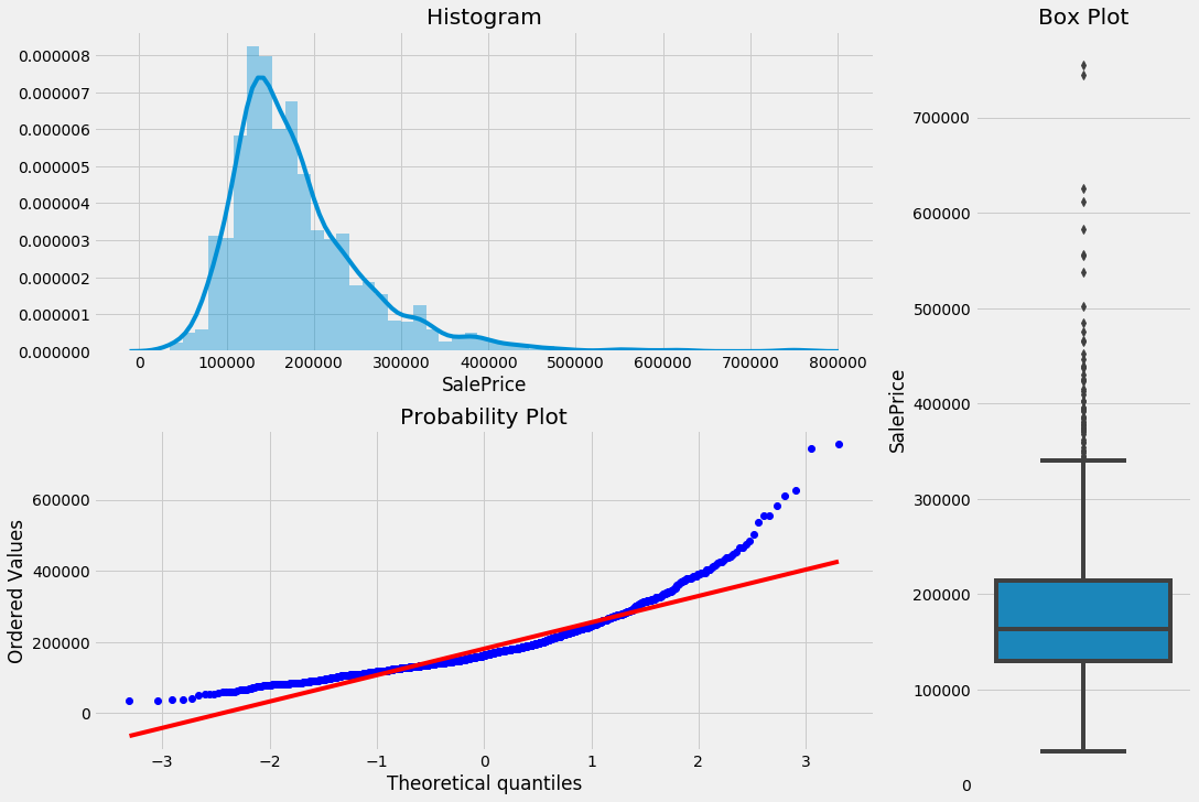
These three charts above can tell us a lot about our target variable.
- Our target variable, SalePrice is not normally distributed.
- Our target variable is right-skewed.
- There are multiple outliers in the variable.
#skewness and kurtosis
print("Skewness: " + str(train['SalePrice'].skew()))
print("Kurtosis: " + str(train['SalePrice'].kurt()))
Skewness: 1.8828757597682129
Kurtosis: 6.536281860064529
## trainsforming target variable using numpy.log1p,
train["SalePrice"] = np.log1p(train["SalePrice"])

## Plotting the newly transformed response variable
plotting_3_chart(train, 'SalePrice')
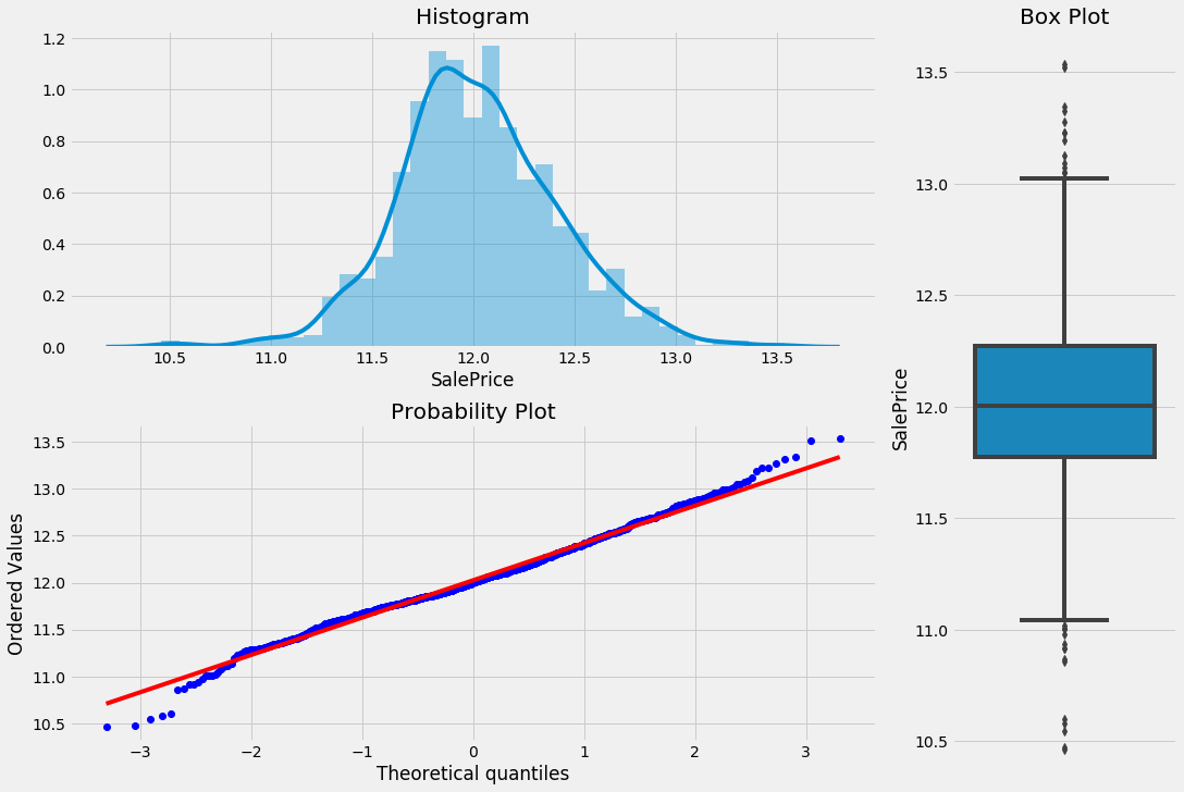
As you can see the log transformation removes the normality of errors. This solves some of the other assumptions that we talked about above like Homoscedasticity. Let’s make a comparison of the pre-transformed and post-transformed state of residual plots.
## Customizing grid for two plots.
fig, (ax1, ax2) = plt.subplots(figsize = (20,6), ncols=2, sharey = False, sharex=False)
## doing the first scatter plot.
sns.residplot(x = previous_train.GrLivArea, y = previous_train.SalePrice, ax = ax1)
## doing the scatter plot for GrLivArea and SalePrice.
sns.residplot(x = train.GrLivArea, y = train.SalePrice, ax = ax2);
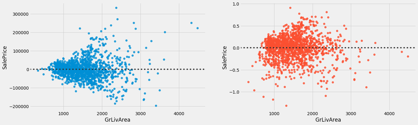
Here, we can see that the pre-transformed chart on the left has heteroscedasticity, and the post-transformed chart on the right has almost an equal amount of variance across the zero lines.
## Plot fig sizing.
style.use('ggplot')
sns.set_style('whitegrid')
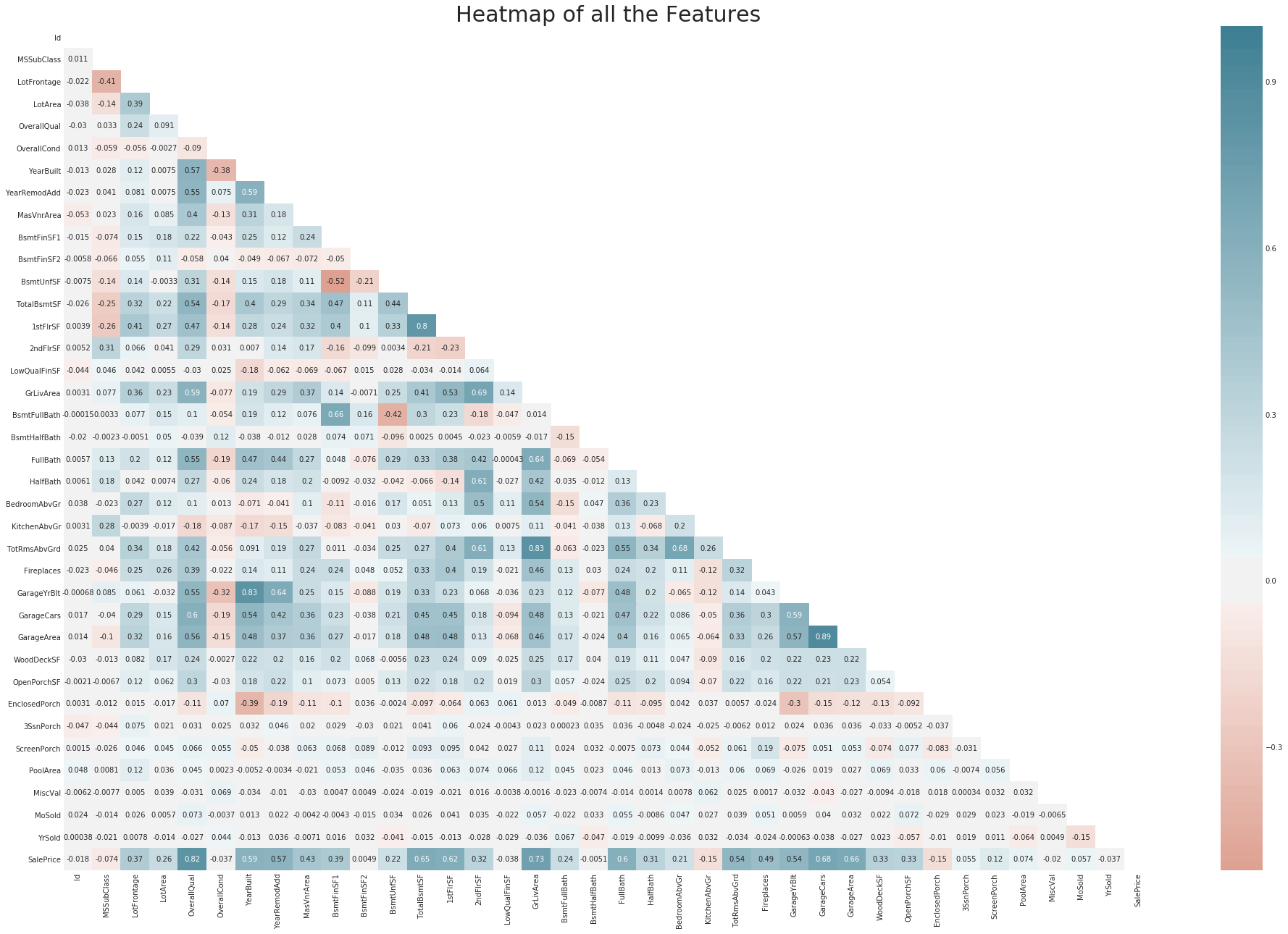
plt.subplots(figsize = (30,20))
## Plotting heatmap.
# Generate a mask for the upper triangle (taken from seaborn example gallery)
mask = np.zeros_like(train.corr(), dtype=np.bool)
mask[np.triu_indices_from(mask)] = True
sns.heatmap(train.corr(), cmap=sns.diverging_palette(20, 220, n=200), mask = mask, annot=True, center = 0, );
## Give title.
plt.title("Heatmap of all the Features", fontsize = 30);
## Dropping the "Id" from train and test set.
# train.drop(columns=['Id'],axis=1, inplace=True)

train.drop(columns=['Id'],axis=1, inplace=True)
test.drop(columns=['Id'],axis=1, inplace=True)

## Saving the target values in "y_train".
y = train['SalePrice'].reset_index(drop=True)


# getting a copy of train
previous_train = train.copy()
## Combining train and test datasets together so that we can do all the work at once.
all_data = pd.concat((train, test)).reset_index(drop = True)
## Dropping the target variable.
all_data.drop(['SalePrice'], axis = 1, inplace = True)
Dealing with Missing Values
Missing data in train and test data(all_data)
Imputing Missing Values
## Some missing values are intentionally left blank, for example: In the Alley feature
## there are blank values meaning that there are no alley's in that specific house.
missing_val_col = ["Alley",
                   "PoolQC",
                   "MiscFeature",
                   "Fence",
                   "FireplaceQu",
                   "GarageType",
                   "GarageFinish",
                   "GarageQual",
                   "GarageCond",
                   'BsmtQual',
                   'BsmtCond',
                   'BsmtExposure',
                   'BsmtFinType1',
                   'BsmtFinType2',
                   'MasVnrType']

for i in missing_val_col:
    all_data[i] = all_data[i].fillna('None')
## These features are continous variable, we used "0" to replace the null values.
missing_val_col2 = ['BsmtFinSF1',
                    'BsmtFinSF2',
                    'BsmtUnfSF',
                    'TotalBsmtSF',
                    'BsmtFullBath',
                    'BsmtHalfBath',
                    'GarageYrBlt',
                    'GarageArea',
                    'GarageCars',
                    'MasVnrArea']

for i in missing_val_col2:
    all_data[i] = all_data[i].fillna(0)

## Replaced all missing values in LotFrontage by imputing the median value of each neighborhood.
all_data['LotFrontage'] = all_data.groupby('Neighborhood')['LotFrontage'].transform( lambda x: x.fillna(x.mean()))
## the "OverallCond" and "OverallQual" of the house.
# all_data['OverallCond'] = all_data['OverallCond'].astype(str)
# all_data['OverallQual'] = all_data['OverallQual'].astype(str)

## Zoning class are given in numerical; therefore converted to categorical variables.
all_data['MSSubClass'] = all_data['MSSubClass'].astype(str)
all_data['MSZoning'] = all_data.groupby('MSSubClass')['MSZoning'].transform(lambda x: x.fillna(x.mode()[0]))

## Important years and months that should be categorical variables not numerical.
# all_data['YearBuilt'] = all_data['YearBuilt'].astype(str)
# all_data['YearRemodAdd'] = all_data['YearRemodAdd'].astype(str)
# all_data['GarageYrBlt'] = all_data['GarageYrBlt'].astype(str)
all_data['YrSold'] = all_data['YrSold'].astype(str)
all_data['MoSold'] = all_data['MoSold'].astype(str)
all_data['Functional'] = all_data['Functional'].fillna('Typ')
all_data['Utilities'] = all_data['Utilities'].fillna('AllPub')
all_data['Exterior1st'] = all_data['Exterior1st'].fillna(all_data['Exterior1st'].mode()[0])
all_data['Exterior2nd'] = all_data['Exterior2nd'].fillna(all_data['Exterior2nd'].mode()[0])
all_data['KitchenQual'] = all_data['KitchenQual'].fillna("TA")
all_data['SaleType'] = all_data['SaleType'].fillna(all_data['SaleType'].mode()[0])
all_data['Electrical'] = all_data['Electrical'].fillna("SBrkr")
missing_percentage(all_data)
| Total | Percent |
|---|
So, there are no missing value left.
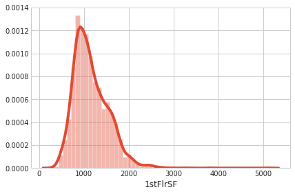
sns.distplot(all_data['1stFlrSF']);
numeric_feats = all_data.dtypes[all_data.dtypes != "object"].index

skewed_feats = all_data[numeric_feats].apply(lambda x: skew(x)).sort_values(ascending=False)

skewed_feats
MiscVal          21.939672
PoolArea         17.688664
LotArea          13.109495
LowQualFinSF     12.084539
3SsnPorch        11.372080
KitchenAbvGr      4.300550
BsmtFinSF2        4.144503
EnclosedPorch     4.002344
ScreenPorch       3.945101
BsmtHalfBath      3.929996
MasVnrArea        2.621719
OpenPorchSF       2.529358
WoodDeckSF        1.844792
1stFlrSF          1.257286
GrLivArea         1.068750
LotFrontage       1.058803
BsmtFinSF1        0.980645
BsmtUnfSF         0.919688
2ndFlrSF          0.861556
TotRmsAbvGrd      0.749232
Fireplaces        0.725278
HalfBath          0.696666
TotalBsmtSF       0.671751
BsmtFullBath      0.622415
OverallCond       0.569314
BedroomAbvGr      0.326568
GarageArea        0.216857
OverallQual       0.189591
FullBath          0.165514
GarageCars       -0.219297
YearRemodAdd     -0.450134
YearBuilt        -0.599194
GarageYrBlt      -3.904632
dtype: float64
## Fixing Skewed features using boxcox transformation.
def fixing_skewness(df):
"""
This function takes in a dataframe and return fixed skewed dataframe
"""
## Import necessary modules
from scipy.stats import skew
from scipy.special import boxcox1p
from scipy.stats import boxcox_normmax
## Getting all the data that are not of "object" type.
numeric_feats = df.dtypes[df.dtypes != "object"].index
# Check the skew of all numerical features
skewed_feats = df[numeric_feats].apply(lambda x: skew(x)).sort_values(ascending=False)
high_skew = skewed_feats[abs(skewed_feats) > 0.5]
skewed_features = high_skew.index
for feat in skewed_features:
df[feat] = boxcox1p(df[feat], boxcox_normmax(df[feat] + 1))
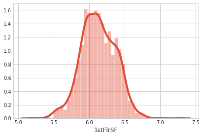
fixing_skewness(all_data)
sns.distplot(all_data['1stFlrSF']);
all_data = all_data.drop(['Utilities', 'Street', 'PoolQC',], axis=1)

# feture engineering a new feature "TotalFS"
all_data['TotalSF'] = all_data['TotalBsmtSF'] + all_data['1stFlrSF'] + all_data['2ndFlrSF']
all_data['YrBltAndRemod']=all_data['YearBuilt']+all_data['YearRemodAdd']

all_data['Total_sqr_footage'] = (all_data['BsmtFinSF1'] + all_data['BsmtFinSF2'] +
                                 all_data['1stFlrSF'] + all_data['2ndFlrSF'])

all_data['Total_Bathrooms'] = (all_data['FullBath'] + (0.5 * all_data['HalfBath']) +
                               all_data['BsmtFullBath'] + (0.5 * all_data['BsmtHalfBath']))

all_data['Total_porch_sf'] = (all_data['OpenPorchSF'] + all_data['3SsnPorch'] +
                              all_data['EnclosedPorch'] + all_data['ScreenPorch'] +
                              all_data['WoodDeckSF'])
all_data['haspool'] = all_data['PoolArea'].apply(lambda x: 1 if x > 0 else 0)
all_data['has2ndfloor'] = all_data['2ndFlrSF'].apply(lambda x: 1 if x > 0 else 0)
all_data['hasgarage'] = all_data['GarageArea'].apply(lambda x: 1 if x > 0 else 0)
all_data['hasbsmt'] = all_data['TotalBsmtSF'].apply(lambda x: 1 if x > 0 else 0)
all_data['hasfireplace'] = all_data['Fireplaces'].apply(lambda x: 1 if x > 0 else 0)
all_data.shape
(2917, 86)
Creating Dummy Variables.
## Creating dummy variable
final_features = pd.get_dummies(all_data).reset_index(drop=True)
final_features.shape
(2917, 333)
X = final_features.iloc[:len(y), :]

X_sub = final_features.iloc[len(y):, :]
outliers = [30, 88, 462, 631, 1322]
X = X.drop(X.index[outliers])
y = y.drop(y.index[outliers])
def overfit_reducer(df):
    """
    This function takes in a dataframe and returns a list of features that are overfitted.
    """
    overfit = []
    for i in df.columns:
        counts = df[i].value_counts()
        zeros = counts.iloc[0]
        if zeros / len(df) * 100 > 99.94:
            overfit.append(i)
    overfit = list(overfit)
    return overfit


overfitted_features = overfit_reducer(X)

X = X.drop(overfitted_features, axis=1)
X_sub = X_sub.drop(overfitted_features, axis=1)
X.shape,y.shape, X_sub.shape
((1453, 332), (1453,), (1459, 332))
Fitting model(simple approach)
Train_test split
## Train test s
from sklearn.model_selection import train_test_split
## Train test split follows this distinguished code pattern and helps creating train and test set to build machine learning.
X_train, X_test, y_train, y_test = train_test_split(X, y,test_size = .33, random_state = 0)
X_train.shape, y_train.shape, X_test.shape, y_test.shape
((973, 332), (973,), (480, 332), (480,))
Regularization Models
What makes regression model more effective is its ability of regularizing. The term “regularizing” stands for models ability to structurally prevent overfitting by imposing a penalty on the coefficients.
There are three types of regularizations.
- Ridge
- Lasso
- Elastic Net
Ridge:
Ridge regression adds penalty equivalent to the square of the magnitude of the coefficients. This penalty is added to the least square loss function above and looks like this…
## Importing Ridge.
from sklearn.linear_model import Ridge
from sklearn.metrics import mean_absolute_error, mean_squared_error
## Assiging different sets of alpha values to explore which can be the best fit for the model.
alpha_ridge = [-3,-2,-1,1e-15, 1e-10, 1e-8,1e-5,1e-4, 1e-3,1e-2,0.5,1,1.5, 2,3,4, 5, 10, 20, 30, 40]
temp_rss = {}
temp_mse = {}
for i in alpha_ridge:
    ## Assigin each model.
    ridge = Ridge(alpha= i, normalize=True)
    ## fit the model.
    ridge.fit(X_train, y_train)
    ## Predicting the target value based on "Test_x"
    y_pred = ridge.predict(X_test)

    mse = mean_squared_error(y_test, y_pred)
    rss = sum((y_pred-y_test)**2)
    temp_mse[i] = mse
    temp_rss[i] = rss
for key, value in sorted(temp_mse.items(), key=lambda item: item[1]):
    print("%s: %s" % (key, value))
0.01: 0.012058094362558029
0.001: 0.012361806597259932
0.5: 0.012398339976451882
0.0001: 0.01245484128284161
1e-05: 0.012608710731947215
1e-15: 0.0126876442980313
1e-08: 0.012689390127616456
1e-10: 0.012689491191917741
1: 0.013828461568989092
1.5: 0.015292912807173023
2: 0.016759826630923253
3: 0.019679216533917247
4: 0.02256515576039871
5: 0.02540603527247574
10: 0.03869750099582716
20: 0.06016951688745736
30: 0.07597213357728104
40: 0.08783870545120151
-1: 22.58422122267688
-3: 37.77842304072701
-2: 1127.9896486631667
for key, value in sorted(temp_rss.items(), key=lambda item: item[1]):
    print("%s: %s" % (key, value))
0.01: 5.787885294027853
0.001: 5.9336671666847645
0.5: 5.951203188696909
0.0001: 5.978323815763974
1e-05: 6.052181151334658
1e-15: 6.090069263055022
1e-08: 6.090907261255897
1e-10: 6.09095577212052
1: 6.637661553114765
1.5: 7.34059814744305
2: 8.044716782843166
3: 9.446023936280277
4: 10.831274764991383
5: 12.194896930788355
10: 18.574800477997016
20: 28.881368105979536
30: 36.46662411709491
40: 42.16257861657673
-1: 10840.426186884908
-3: 18133.64305954895
-2: 541435.0313583203
Lasso:
Lasso adds penalty equivalent to the absolute value of the sum of coefficients. This penalty is added to the least square loss function and replaces the squared sum of coefficients from Ridge.
from sklearn.linear_model import Lasso
temp_rss = {}
temp_mse = {}
for i in alpha_ridge:
    ## Assigin each model.
    lasso_reg = Lasso(alpha= i, normalize=True)
    ## fit the model.
    lasso_reg.fit(X_train, y_train)
    ## Predicting the target value based on "Test_x"
    y_pred = lasso_reg.predict(X_test)

    mse = mean_squared_error(y_test, y_pred)
    rss = sum((y_pred-y_test)**2)
    temp_mse[i] = mse
    temp_rss[i] = rss
for key, value in sorted(temp_mse.items(), key=lambda item: item[1]):
    print("%s: %s" % (key, value))
0.0001: 0.010061658258835855
1e-05: 0.011553103092552693
1e-08: 0.012464777509974378
1e-10: 0.012469892082710245
1e-15: 0.01246993993780167
0.001: 0.01834391027644981
0.01: 0.15998234085337285
0.5: 0.16529633945001213
1: 0.16529633945001213
1.5: 0.16529633945001213
2: 0.16529633945001213
3: 0.16529633945001213
4: 0.16529633945001213
5: 0.16529633945001213
10: 0.16529633945001213
20: 0.16529633945001213
30: 0.16529633945001213
40: 0.16529633945001213
-1: 14648689598.250006
-2: 58594759730.8125
-3: 131838210397.70003
for key, value in sorted(temp_rss.items(), key=lambda item: item[1]):
    print("%s: %s" % (key, value))
0.0001: 4.82959596424121
1e-05: 5.545489484425293
1e-08: 5.9830932047877035
1e-10: 5.985548199700918
1e-15: 5.9855711701448
0.001: 8.805076932695897
0.01: 76.79152360961895
0.5: 79.34224293600582
1: 79.34224293600582
1.5: 79.34224293600582
2: 79.34224293600582
3: 79.34224293600582
4: 79.34224293600582
5: 79.34224293600582
10: 79.34224293600582
20: 79.34224293600582
30: 79.34224293600582
40: 79.34224293600582
-1: 7031371007160.002
-2: 28125484670789.992
-3: 63282340990896.01
Elastic Net:
Elastic Net is the combination of both Ridge and Lasso. It adds both the sum of squared coefficients and the absolute sum of the coefficients with the ordinary least square function. Let’s look at the function.
from sklearn.linear_model import ElasticNet
temp_rss = {}
temp_mse = {}
for i in alpha_ridge:
    ## Assigin each model.
    lasso_reg = ElasticNet(alpha= i, normalize=True)
    ## fit the model.
    lasso_reg.fit(X_train, y_train)
    ## Predicting the target value based on "Test_x"
    y_pred = lasso_reg.predict(X_test)

    mse = mean_squared_error(y_test, y_pred)
    rss = sum((y_pred-y_test)**2)
    temp_mse[i] = mse
    temp_rss[i] = rss
for key, value in sorted(temp_mse.items(), key=lambda item: item[1]):
    print("%s: %s" % (key, value))
0.0001: 0.010410247442255985
1e-05: 0.011786774263401294
1e-08: 0.012466548787037617
1e-10: 0.012469905615434403
1e-15: 0.012469939937937151
0.001: 0.014971538718578314
0.01: 0.10870291488354142
0.5: 0.16529633945001213
1: 0.16529633945001213
1.5: 0.16529633945001213
2: 0.16529633945001213
3: 0.16529633945001213
4: 0.16529633945001213
5: 0.16529633945001213
10: 0.16529633945001213
20: 0.16529633945001213
30: 0.16529633945001213
40: 0.16529633945001213
-3: 5.388825733568653
-2: 5.470945111059094
-1: 5.729175782943725
for key, value in sorted(temp_rss.items(), key=lambda item: item[1]):
    print("%s: %s" % (key, value))
0.0001: 4.996918772282872
1e-05: 5.65765164643262
1e-08: 5.983943417778055
1e-10: 5.985554695408507
1e-15: 5.9855711702098295
0.001: 7.186338584917596
0.01: 52.17739914409985
0.5: 79.34224293600582
1: 79.34224293600582
1.5: 79.34224293600582
2: 79.34224293600582
3: 79.34224293600582
4: 79.34224293600582
5: 79.34224293600582
10: 79.34224293600582
20: 79.34224293600582
30: 79.34224293600582
40: 79.34224293600582
-3: 2586.6363521129515
-2: 2626.053653308364
-1: 2750.0043758129887
Fitting model (Advanced approach)
kfolds = KFold(n_splits=10, shuffle=True, random_state=42)

def rmsle(y, y_pred):
    return np.sqrt(mean_squared_error(y, y_pred))

def cv_rmse(model, X=X):
    rmse = np.sqrt(-cross_val_score(model, X, y, scoring="neg_mean_squared_error", cv=kfolds))
    return (rmse)
alphas_alt = [14.5, 14.6, 14.7, 14.8, 14.9, 15, 15.1, 15.2, 15.3, 15.4, 15.5]
alphas2 = [5e-05, 0.0001, 0.0002, 0.0003, 0.0004, 0.0005, 0.0006, 0.0007, 0.0008]
e_alphas = [0.0001, 0.0002, 0.0003, 0.0004, 0.0005, 0.0006, 0.0007]
e_l1ratio = [0.8, 0.85, 0.9, 0.95, 0.99, 1]
ridge = make_pipeline(RobustScaler(), RidgeCV(alphas=alphas_alt, cv=kfolds))
lasso = make_pipeline(RobustScaler(), LassoCV(max_iter=1e7, alphas=alphas2, random_state=42, cv=kfolds))
elasticnet = make_pipeline(RobustScaler(), ElasticNetCV(max_iter=1e7, alphas=e_alphas, cv=kfolds, l1_ratio=e_l1ratio))
svr = make_pipeline(RobustScaler(), SVR(C= 20, epsilon= 0.008, gamma=0.0003,))
gbr = GradientBoostingRegressor(n_estimators=3000, learning_rate=0.05, max_depth=4, max_features='sqrt', min_samples_leaf=15, min_samples_split=10, loss='huber', random_state =42)
lightgbm = LGBMRegressor(objective='regression',
                                       num_leaves=4,
                                       learning_rate=0.01,
                                       n_estimators=5000,
                                       max_bin=200,
                                       bagging_fraction=0.75,
                                       bagging_freq=5,
                                       bagging_seed=7,
                                       feature_fraction=0.2,
                                       feature_fraction_seed=7,
                                       verbose=-1,
                                       )
xgboost = XGBRegressor(learning_rate=0.01,n_estimators=3460,
                                     max_depth=3, min_child_weight=0,
                                     gamma=0, subsample=0.7,
                                     colsample_bytree=0.7,
                                     objective='reg:linear', nthread=-1,
                                     scale_pos_weight=1, seed=27,
                                     reg_alpha=0.00006)
stack_gen = StackingCVRegressor(regressors=(ridge, lasso, elasticnet, xgboost, lightgbm),
                                meta_regressor=xgboost,
                                use_features_in_secondary=True)
# score = cv_rmse(stack_gen)
score = cv_rmse(ridge)
print("Ridge: {:.4f} ({:.4f})\n".format(score.mean(), score.std()), datetime.now(), )

score = cv_rmse(lasso)
print("LASSO: {:.4f} ({:.4f})\n".format(score.mean(), score.std()), datetime.now(), )

score = cv_rmse(elasticnet)
print("elastic net: {:.4f} ({:.4f})\n".format(score.mean(), score.std()), datetime.now(), )

score = cv_rmse(svr)
print("SVR: {:.4f} ({:.4f})\n".format(score.mean(), score.std()), datetime.now(), )

score = cv_rmse(lightgbm)
print("lightgbm: {:.4f} ({:.4f})\n".format(score.mean(), score.std()), datetime.now(), )

# score = cv_rmse(gbr)
# print("gbr: {:.4f} ({:.4f})\n".format(score.mean(), score.std()), datetime.now(), )

score = cv_rmse(xgboost)
print("xgboost: {:.4f} ({:.4f})\n".format(score.mean(), score.std()), datetime.now(), )
Ridge: 0.1011 (0.0141)
 2020-01-22 15:12:38.941969
LASSO: 0.0997 (0.0142)
 2020-01-22 15:12:45.519931
elastic net: 0.0998 (0.0143)
 2020-01-22 15:13:12.882048
SVR: 0.1020 (0.0146)
 2020-01-22 15:13:26.262319
lightgbm: 0.1054 (0.0154)
 2020-01-22 15:13:44.348901
[15:13:44] WARNING: /workspace/src/objective/regression_obj.cu:152: reg:linear is now deprecated in favor of reg:squarederror.
[15:13:58] WARNING: /workspace/src/objective/regression_obj.cu:152: reg:linear is now deprecated in favor of reg:squarederror.
[15:14:12] WARNING: /workspace/src/objective/regression_obj.cu:152: reg:linear is now deprecated in favor of reg:squarederror.
[15:14:28] WARNING: /workspace/src/objective/regression_obj.cu:152: reg:linear is now deprecated in favor of reg:squarederror.
[15:14:42] WARNING: /workspace/src/objective/regression_obj.cu:152: reg:linear is now deprecated in favor of reg:squarederror.
[15:14:55] WARNING: /workspace/src/objective/regression_obj.cu:152: reg:linear is now deprecated in favor of reg:squarederror.
[15:15:09] WARNING: /workspace/src/objective/regression_obj.cu:152: reg:linear is now deprecated in favor of reg:squarederror.
[15:15:25] WARNING: /workspace/src/objective/regression_obj.cu:152: reg:linear is now deprecated in favor of reg:squarederror.
[15:15:39] WARNING: /workspace/src/objective/regression_obj.cu:152: reg:linear is now deprecated in favor of reg:squarederror.
[15:15:53] WARNING: /workspace/src/objective/regression_obj.cu:152: reg:linear is now deprecated in favor of reg:squarederror.
xgboost: 0.1061 (0.0147)
 2020-01-22 15:16:07.581332
print('START Fit')

print('stack_gen')
stack_gen_model = stack_gen.fit(np.array(X), np.array(y))

print('elasticnet')
elastic_model_full_data = elasticnet.fit(X, y)

print('Lasso')
lasso_model_full_data = lasso.fit(X, y)

print('Ridge')
ridge_model_full_data = ridge.fit(X, y)

print('Svr')
svr_model_full_data = svr.fit(X, y)

# print('GradientBoosting')
# gbr_model_full_data = gbr.fit(X, y)

print('xgboost')
xgb_model_full_data = xgboost.fit(X, y)

print('lightgbm')
lgb_model_full_data = lightgbm.fit(X, y)
START Fit
stack_gen
[15:17:42] WARNING: /workspace/src/objective/regression_obj.cu:152: reg:linear is now deprecated in favor of reg:squarederror.
[15:17:54] WARNING: /workspace/src/objective/regression_obj.cu:152: reg:linear is now deprecated in favor of reg:squarederror.
[15:18:07] WARNING: /workspace/src/objective/regression_obj.cu:152: reg:linear is now deprecated in favor of reg:squarederror.
[15:18:21] WARNING: /workspace/src/objective/regression_obj.cu:152: reg:linear is now deprecated in favor of reg:squarederror.
[15:18:34] WARNING: /workspace/src/objective/regression_obj.cu:152: reg:linear is now deprecated in favor of reg:squarederror.
[15:18:54] WARNING: /workspace/src/objective/regression_obj.cu:152: reg:linear is now deprecated in favor of reg:squarederror.
[15:19:15] WARNING: /workspace/src/objective/regression_obj.cu:152: reg:linear is now deprecated in favor of reg:squarederror.
elasticnet
Lasso
Ridge
Svr
xgboost
[15:19:40] WARNING: /workspace/src/objective/regression_obj.cu:152: reg:linear is now deprecated in favor of reg:squarederror.
lightgbm
Blending Models
1.0 * elastic_model_full_data.predict(X)
array([12.2252765 , 12.19482971, 12.28743582, ..., 12.45057568,
       11.846052  , 11.9162269 ])
def blend_models_predict(X):
    return ((0.1 * elastic_model_full_data.predict(X)) + \
            (0.05 * lasso_model_full_data.predict(X)) + \
            (0.2 * ridge_model_full_data.predict(X)) + \
            (0.1 * svr_model_full_data.predict(X)) + \
#             (0.1 * gbr_model_full_data.predict(X)) + \
            (0.15 * xgb_model_full_data.predict(X)) + \
            (0.1 * lgb_model_full_data.predict(X)) + \
            (0.3 * stack_gen_model.predict(np.array(X))))
print('RMSLE score on train data:')
print(rmsle(y, blend_models_predict(X)))
RMSLE score on train data:
0.06279142797823006
submission = pd.read_csv("../input/house-prices-advanced-regression-techniques/sample_submission.csv")
submission.iloc[:,1] = np.floor(np.expm1(blend_models_predict(X_sub)))
Predict submission
Submission
q1 = submission['SalePrice'].quantile(0.005)
q2 = submission['SalePrice'].quantile(0.995)
submission['SalePrice'] = submission['SalePrice'].apply(lambda x: x if x > q1 else x*0.77)
submission['SalePrice'] = submission['SalePrice'].apply(lambda x: x if x < q2 else x*1.1)
submission.to_csv("submission.csv", index=False)
Reference
Notebooks in kaggle:
House Prices: 1st Approach to Data Science Process
Stack&Blend LRs XGB LGB {House Prices K} v17