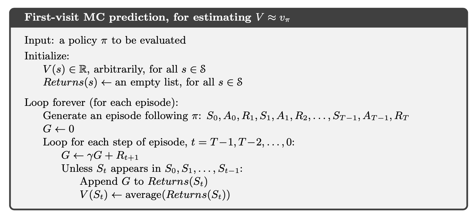
First-Visit Monte Carlo(MC) method: estimate \(v_\pi(s)\) as the average of the returns following the first visit to \(s\). An example of first-visit MC prediction algorithm is shown below:

Implementation of Example 5.1 Blackjack

The object of the popular casino card game of blackjack is to obtain cards the sum of whose numerical values is as great as possible without exceeding 21. All face cards count as 10, and an ace can count either as 1 or as 11. We consider the version in which each player competes independently against the dealer. The game begins with two cards dealt to both dealer and player. One of the dealer’s cards is face up and the other is face down. If the player has 21 immediately (an ace and a 10-card), it is called a natural. He then wins unless the dealer also has a natural, in which case the game is a draw. If the player does not have a natural, then he can request additional cards, one by one (hits), until he either stops (sticks) or exceeds 21 (goes bust). If he goes bust, he loses; if he sticks, then it becomes the dealer’s turn. The dealer hits or sticks according to a fixed strategy without choice: he sticks on any sum of 17 or greater, and hits otherwise. If the dealer goes bust, then the player wins; otherwise, the outcome—win, lose, or draw—is determined by whose final sum is closer to 21. Playing blackjack is naturally formulated as an episodic finite MDP. Each game of blackjack is an episode. Rewards of +1, 1, and 0 are given for winning, losing, and drawing, respectively. All rewards within a game are zero, and we do not discount ($\gamma$= 1); therefore these terminal rewards are also the returns. The player’s actions are to hit or to stick. The states depend on the player’s cards and the dealer’s showing card. We assume that cards are dealt from an infinite deck (i.e., with replacement) so that there is no advantage to keeping track of the cards already dealt. If the player holds an ace that he could count as 11 without going bust, then the ace is said to be usable. In this case it is always counted as 11 because counting it as 1 would make the sum 11 or less, in which case there is no decision to be made because, obviously, the player should always hit. Thus, the player makes decisions on the basis of three variables: his current sum (12–21), the dealer’s one showing card (ace–10), and whether or not he holds a usable ace. This makes for a total of 200 states. Consider the policy that sticks if the player’s sum is 20 or 21, and otherwise hits. To find the state-value function for this policy by a Monte Carlo approach, one simulates many blackjack games using the policy and averages the returns following each state. In this way, we obtained the estimates of the state-value function shown in Figure 5.1. The estimates for states with a usable ace are less certain and less regular because these states are less common. In any event, after 500,000 games the value function is very well approximated.

import numpy as np
import matplotlib
import matplotlib.pyplot as plt
%matplotlib inline
import seaborn as sns
from tqdm import tqdm
import warnings
warnings.filterwarnings('ignore')

# actions: hit or stand
ACTION_HIT = 0
ACTION_STAND = 1  #  "strike" in the book
ACTIONS = [ACTION_HIT, ACTION_STAND]

# policy for player
POLICY_PLAYER = np.zeros(22, dtype=np.int)
for i in range(12, 20):
    POLICY_PLAYER[i] = ACTION_HIT
POLICY_PLAYER[20] = ACTION_STAND
POLICY_PLAYER[21] = ACTION_STAND

# function form of target policy of player
def target_policy_player(usable_ace_player, player_sum, dealer_card):
    return POLICY_PLAYER[player_sum]

# function form of behavior policy of player
def behavior_policy_player(usable_ace_player, player_sum, dealer_card):
    if np.random.binomial(1, 0.5) == 1:
        return ACTION_STAND
    return ACTION_HIT

# policy for dealer
POLICY_DEALER = np.zeros(22)
for i in range(12, 17):
    POLICY_DEALER[i] = ACTION_HIT
for i in range(17, 22):
    POLICY_DEALER[i] = ACTION_STAND

# get a new card
def get_card():
    card = np.random.randint(1, 14)
    card = min(card, 10)
    return card

# get the value of a card (11 for ace).
def card_value(card_id):
    return 11 if card_id == 1 else card_id

# play a game
# @policy_player: specify policy for player
# @initial_state: [whether player has a usable Ace, sum of player's cards, one card of dealer]
# @initial_action: the initial action
def play(policy_player, initial_state=None, initial_action=None):
    # player status

    # sum of player
    player_sum = 0

    # trajectory of player
    player_trajectory = []

    # whether player uses Ace as 11
    usable_ace_player = False

    # dealer status
    dealer_card1 = 0
    dealer_card2 = 0
    usable_ace_dealer = False

    if initial_state is None:
        # generate a random initial state

        while player_sum < 12:
            # if sum of player is less than 12, always hit
            card = get_card()
            player_sum += card_value(card)

            # If the player's sum is larger than 21, he may hold one or two aces.
            if player_sum > 21:
                assert player_sum == 22
                # last card must be ace
                player_sum -= 10
            else:
                # usable_ace_player = usable_ace_player | (1 == card)
                usable_ace_player |= (1 == card)

        # initialize cards of dealer, suppose dealer will show the first card he gets
        dealer_card1 = get_card()
        dealer_card2 = get_card()

    else:
        # use specified initial state
        usable_ace_player, player_sum, dealer_card1 = initial_state
        dealer_card2 = get_card()

    # initial state of the game
    state = [usable_ace_player, player_sum, dealer_card1]

    # initialize dealer's sum
    dealer_sum = card_value(dealer_card1) + card_value(dealer_card2)
    usable_ace_dealer = 1 in (dealer_card1, dealer_card2)
    # if the dealer's sum is larger than 21, he must hold two aces.
    if dealer_sum > 21:
        assert dealer_sum == 22
        # use one Ace as 1 rather than 11
        dealer_sum -= 10
    assert dealer_sum <= 21
    assert player_sum <= 21

    # game starts!

    # player's turn
    while True:
        if initial_action is not None:
            action = initial_action
            initial_action = None
        else:
            # get action based on current sum
            action = policy_player(usable_ace_player, player_sum, dealer_card1)

        # track player's trajectory for importance sampling
        player_trajectory.append([(usable_ace_player, player_sum, dealer_card1), action])

        if action == ACTION_STAND:
            break
        # if hit, get new card
        card = get_card()
        # Keep track of the ace count. the usable_ace_player flag is insufficient alone as it cannot
        # distinguish between having one ace or two.
        ace_count = int(usable_ace_player)
        if card == 1:
            ace_count += 1
        player_sum += card_value(card)
        # If the player has a usable ace, use it as 1 to avoid busting and continue.
        while player_sum > 21 and ace_count:
            player_sum -= 10
            ace_count -= 1
        # player busts
        if player_sum > 21:
            return state, -1, player_trajectory
        assert player_sum <= 21
        usable_ace_player = (ace_count == 1)

    # dealer's turn
    while True:
        # get action based on current sum
        action = POLICY_DEALER[dealer_sum]
        if action == ACTION_STAND:
            break
        # if hit, get a new card
        new_card = get_card()
        ace_count = int(usable_ace_dealer)
        if new_card == 1:
            ace_count += 1
        dealer_sum += card_value(new_card)
        # If the dealer has a usable ace, use it as 1 to avoid busting and continue.
        while dealer_sum > 21 and ace_count:
            dealer_sum -= 10
            ace_count -= 1
        # dealer busts
        if dealer_sum > 21:
            return state, 1, player_trajectory
        usable_ace_dealer = (ace_count == 1)

    # compare the sum between player and dealer
    assert player_sum <= 21 and dealer_sum <= 21
    if player_sum > dealer_sum:
        return state, 1, player_trajectory
    elif player_sum == dealer_sum:
        return state, 0, player_trajectory
    else:
        return state, -1, player_trajectory

# Monte Carlo Sample with On-Policy
def monte_carlo_on_policy(episodes):
    states_usable_ace = np.zeros((10, 10))
    # initialze counts to 1 to avoid 0 being divided
    states_usable_ace_count = np.ones((10, 10))
    states_no_usable_ace = np.zeros((10, 10))
    # initialze counts to 1 to avoid 0 being divided
    states_no_usable_ace_count = np.ones((10, 10))
    for i in tqdm(range(0, episodes)):
        _, reward, player_trajectory = play(target_policy_player)
        for (usable_ace, player_sum, dealer_card), _ in player_trajectory:
            player_sum -= 12
            dealer_card -= 1
            if usable_ace:
                states_usable_ace_count[player_sum, dealer_card] += 1
                states_usable_ace[player_sum, dealer_card] += reward
            else:
                states_no_usable_ace_count[player_sum, dealer_card] += 1
                states_no_usable_ace[player_sum, dealer_card] += reward
    return states_usable_ace / states_usable_ace_count, states_no_usable_ace / states_no_usable_ace_count

def figure_5_1():
    states_usable_ace_1, states_no_usable_ace_1 = monte_carlo_on_policy(10000)
    states_usable_ace_2, states_no_usable_ace_2 = monte_carlo_on_policy(500000)

    states = [states_usable_ace_1,
              states_usable_ace_2,
              states_no_usable_ace_1,
              states_no_usable_ace_2]

    titles = ['Usable Ace, 10000 Episodes',
              'Usable Ace, 500000 Episodes',
              'No Usable Ace, 10000 Episodes',
              'No Usable Ace, 500000 Episodes']

    _, axes = plt.subplots(2, 2, figsize=(40, 30))
    plt.subplots_adjust(wspace=0.1, hspace=0.2)
    axes = axes.flatten()

    for state, title, axis in zip(states, titles, axes):
        fig = sns.heatmap(np.flipud(state), cmap="YlGnBu", ax=axis, xticklabels=range(1, 11),
                          yticklabels=list(reversed(range(12, 22))))
        fig.set_ylabel('player sum', fontsize=30)
        fig.set_xlabel('dealer showing', fontsize=30)
        fig.set_title(title, fontsize=30)

    plt.plot()

figure_5_1()

100%|██████████| 10000/10000 [00:00<00:00, 48228.52it/s]
100%|██████████| 500000/500000 [00:09<00:00, 53947.10it/s]

By Law of Large Numbers, as number of visits to \(s \rightarrow \infty \Rightarrow \text{ first MC method }\rightarrow v_\pi(s)\)
Estimation of action values: as \(\pi\) is given, we could use exploration by "exploring starts": start in a state-action pair \(\Rightarrow P(\text{select as start})>0\), in order to guarantee all states are visited sufficient times for exploration.
Monte Carlo Control: using GPI, the algorithm is shown below:

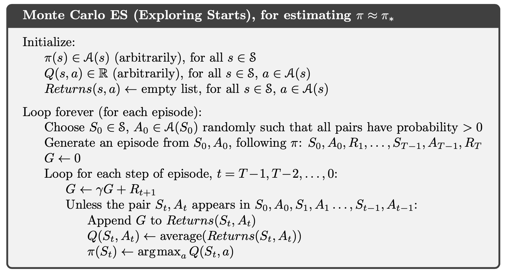
To be efficient and prevent calculating the average every time, we could let $counts(S_t, A_t)\leftarrow counts(S_t, A_t)+1$ and $\displaystyle Q(S_t, A_t)\leftarrow Q(S_t, A_t)+\frac{G-Q(S_t, A_t)}{counts(S_t, A_t)}$ by the update rule in the chapter 2.

Solving the Blackjack

To find the optimal policy:

# Monte Carlo with Exploring Starts
def monte_carlo_es(episodes):
    # (playerSum, dealerCard, usableAce, action)
    state_action_values = np.zeros((10, 10, 2, 2))
    # initialze counts to 1 to avoid division by 0
    state_action_pair_count = np.ones((10, 10, 2, 2))

    # behavior policy is greedy
    def behavior_policy(usable_ace, player_sum, dealer_card):
        usable_ace = int(usable_ace)
        player_sum -= 12
        dealer_card -= 1
        # get argmax of the average returns(s, a)
        values_ = state_action_values[player_sum, dealer_card, usable_ace, :] / \
                  state_action_pair_count[player_sum, dealer_card, usable_ace, :]
        return np.random.choice([action_ for action_, value_ in enumerate(values_) if value_ == np.max(values_)])

    # play for several episodes
    for episode in tqdm(range(episodes)):
        # for each episode, use a randomly initialized state and action
        initial_state = [bool(np.random.choice([0, 1])),
                       np.random.choice(range(12, 22)),
                       np.random.choice(range(1, 11))]
        initial_action = np.random.choice(ACTIONS)
        current_policy = behavior_policy if episode else target_policy_player
        _, reward, trajectory = play(current_policy, initial_state, initial_action)
        first_visit_check = set()
        for (usable_ace, player_sum, dealer_card), action in trajectory:
            usable_ace = int(usable_ace)
            player_sum -= 12
            dealer_card -= 1
            state_action = (usable_ace, player_sum, dealer_card, action)
            if state_action in first_visit_check:
                continue
            first_visit_check.add(state_action)
            # update values of state-action pairs
            state_action_values[player_sum, dealer_card, usable_ace, action] += reward
            state_action_pair_count[player_sum, dealer_card, usable_ace, action] += 1

    return state_action_values / state_action_pair_count

def figure_5_2():
    state_action_values = monte_carlo_es(500000)

    state_value_no_usable_ace = np.max(state_action_values[:, :, 0, :], axis=-1)
    state_value_usable_ace = np.max(state_action_values[:, :, 1, :], axis=-1)

    # get the optimal policy
    action_no_usable_ace = np.argmax(state_action_values[:, :, 0, :], axis=-1)
    action_usable_ace = np.argmax(state_action_values[:, :, 1, :], axis=-1)

    images = [action_usable_ace,
              state_value_usable_ace,
              action_no_usable_ace,
              state_value_no_usable_ace]

    titles = ['Optimal policy with usable Ace',
              'Optimal value with usable Ace',
              'Optimal policy without usable Ace',
              'Optimal value without usable Ace']

    _, axes = plt.subplots(2, 2, figsize=(40, 30))
    plt.subplots_adjust(wspace=0.1, hspace=0.2)
    axes = axes.flatten()

    for image, title, axis in zip(images, titles, axes):
        fig = sns.heatmap(np.flipud(image), cmap="YlGnBu", ax=axis, xticklabels=range(1, 11),
                          yticklabels=list(reversed(range(12, 22))))
        fig.set_ylabel('player sum', fontsize=30)
        fig.set_xlabel('dealer showing', fontsize=30)
        fig.set_title(title, fontsize=30)

    plt.plot()

figure_5_2()

100%|██████████| 500000/500000 [00:41<00:00, 11912.12it/s]

Monte Carlo Control without Exploring Starts

Due to the limitation of the exploration start(e.g. when the agent needs to interact with the environment), Monte Carlo control without exploring starts is introduced next.
on-policy: evaluate and improve the \(\pi\) that is used;
off-policy: evaluate and improve the \(\pi\) that used to;
Then, MC is on-policy. Define "soft": \(\pi(a|s)>0, \forall s\in\mathcal{S}, a\in\mathcal{A}(s)\), but gradually shifted closer and closer to a deterministic optimal policy
\(\epsilon\)-soft greedy: \[\pi^{\prime}(a | s)=\left\{\begin{array}{ll} \frac{\varepsilon}{|\mathcal{A}(s)|} & , \mathbb{P} = \epsilon, \text{non-greedy} \\ 1-\varepsilon-\frac{\varepsilon}{|\mathcal{A}(s)|} & , \mathbb{P} =1- \epsilon, \text{greedy} \end{array}\right.\] Then the on-policy first-visit MC control for \(\epsilon\)-soft policies is shown below:

GPI model requires "becoming greedy" gradually, and from the algorithm above, $\epsilon-$soft policy would become $\epsilon-$greedy policy, and by policy improvement theorem, we can see that greedy method indeed improve the $\epsilon-$soft policy.

Proof:

Let the original $\epsilon-$soft policy $\pi$, with probability distribution:

$\pi\left(a_{i} \mid s\right)=\left\{\begin{array}{ll}\frac{\varepsilon}{|\mathcal{A}(s)|}+\delta_{i} & , a_{i} \neq a_{*} \\ 1-\frac{(|\mathcal{A}(s)|-1) \varepsilon}{|\mathcal{A}(s)|}-\sum_{a_{i} \neq a_{*}} \delta_{i} & , a_{i}=a_{*}\end{array}\right.$

Then,

$\begin{aligned} q_{\pi}(s, \pi^{\prime}) &=\sum_{a} \pi^{\prime}(a \mid s) q_{\pi}(s, a) \\ &=\frac{\varepsilon}{|\mathcal{A}(s)|} \sum_{a} q_{\pi}(s, a)+(1-\varepsilon) \max _{a} q_{\pi}(s, a) \\ &\geq \frac{\varepsilon}{|\mathcal{A}(s)|} \sum_{a} q_{\pi}(s, a)+(1-\varepsilon) \sum_{a} \frac{\pi(a \mid s)-\frac{\varepsilon}{|\mathcal{A}(s)|}}{1-\varepsilon} q_{\pi}(s, a) \\ &=\frac{\varepsilon}{|\mathcal{A}(s)|} \sum_{a} q_{\pi}(s, a)-\frac{\varepsilon}{|\mathcal{A}(s)|} \sum_{a} q_{\pi}(s, a)+\sum_{a} \pi(a \mid s) q_{\pi}(s, a) \\ &=v_{\pi}(s)\end{aligned}$

To prove that $\max _{a} q_{\pi}(s, a) \geq \displaystyle\sum_{a} \frac{\pi(a \mid s)-\frac{\varepsilon}{|\mathcal{A}(s)|}}{1-\varepsilon} q_{\pi}(s, a)$, let $M = \max _{a} q_{\pi}(s, a) $, and,

$\begin{array}{l} \displaystyle\sum_{a} \frac{\pi(a \mid s)-\frac{\varepsilon}{|\mathcal{A}(s)|}}{1-\varepsilon} q_{\pi}(s, a) \\ =\displaystyle\frac{\pi\left(a_{*} \mid s\right)-\frac{\varepsilon}{|\mathcal{A}(s)|}}{1-\varepsilon} M+\sum_{a_{i} \neq a_{*}} \frac{\pi\left(a_{i} \mid s\right)-\frac{\varepsilon}{|\mathcal{A}(s)|}}{1-\varepsilon} q_{\pi}\left(s, a_{i}\right) \\ =\displaystyle\frac{1-\frac{(|\mathcal{A}(s)|-1) \varepsilon}{|\mathcal{A}(s)|}-\sum_{a_{i} \neq a_{*}} \delta_{i}-\frac{\varepsilon}{|\mathcal{A}(s)|}}{1-\varepsilon} M+\sum_{a_{i} \neq a_{*}} \frac{\delta_{i}}{1-\varepsilon} q_{\pi}\left(s, a_{i}\right) \\ =\displaystyle\frac{1-\varepsilon}{1-\varepsilon} M-\frac{1}{1-\varepsilon} \sum_{a_{i} \neq a_{*}} \delta_{i} M+\frac{1}{1-\varepsilon} \sum_{a_{i} \neq a_{*}} \delta_{i} q_{\pi}\left(s, a_{i}\right) \\ =M-\frac{\sum_{a_{i} \neq a_{*}} \delta_{i}}{1-\varepsilon}\left(M-q_{\pi}\left(s, a_{i}\right)\right) \\ \leq M=\max _{a} q_{\pi}(s, a) \end{array}$

And then by theorem, $v_{\pi^\prime} (s)\geq v_\pi(s)$

Off-policy Prediction via Importance Sampling

Learning control method Dillema: They seek to learn action values conditional on subsequent optimal behavior, but they need to behave non-optimally in order to explore all actions (to find the optimal actions).

The on-policy approach in the preceding section is actually a compromise—it learns action values not for the optimal policy, but for a near-optimal policy that still explores. A more straightforward approach is to use two policies, one that is learned about and that becomes the optimal policy, and one that is more exploratory and is used to generate behavior. The policy being learned about is called the target policy, and the policy used to generate behavior is called the behavior policy. In this case we say that learning is from data “off” the target policy, and the overall process is termed off-policy learning. Off-policy include on-policy methods as the special case in which the target and behavior policies are the same. Off-policy learning is also seen by some as key to learning multi-step predictive models of the world’s dynamics(Section 17.2).

In this section we begin the study of off-policy methods by considering the prediction problem, in which both target and behavior policies are fixed. That is, suppose we wish to estimate $v_{\pi}$ or $q_{\pi}$, but all we have are episodes following another policy $b$, where $b \neq \pi .$ In this case, $\pi$ is the target policy, $b$ is the behavior policy, and both policies are considered fixed and given.

Almost all off-policy methods utilize importance sampling, a general technique for estimating expected values under one distribution given samples from another.

As:

$\begin{aligned} \mathbb{E}_{f}[x] &=\int x f(x) \mathrm{d} x \\ &=\int \frac{x f(x)}{g(x)} g(x) \mathrm{d} x \\ &=\mathbb{E}_{g}\left[\frac{f(x)}{g(x)} x\right] \end{aligned}$

Then, $\displaystyle\rho=\frac{f(x)}{g(x)}$ is importance sampling ratio. Then, consider the given State condition,

$\begin{aligned} \mathbb{E}_{f}[x \mid S=s] &=\int x f(x \mid s) \mathrm{d} x \\ &=\int x \frac{f(x \mid s)}{g(x \mid s)} g(x \mid s) \mathrm{d} x \\ &=\mathbb{E}_{g}\left[x \frac{f(x \mid s)}{g(x \mid s)} \mid S=s\right] \\ &=\mathbb{E}_{g}[\rho x \mid S=s] \end{aligned}$

And,

$\begin{array}{l} \mathrm{P}_{\pi}\left\{A_{t}, S_{t+1}, A_{t+1}, \ldots, S_{T} \mid S_{t}\right\} \\ =\pi\left(A_{t} \mid S_{t}\right) p\left(S_{t+1} \mid S_{t}, A_{t}\right) \pi\left(A_{t+1} \mid S_{t+1}\right) \cdots p\left(S_{T} \mid S_{T-1}, A_{T-1}\right) \\ =\prod_{k=t}^{T-1} \pi\left(A_{k} \mid S_{k}\right) p\left(S_{k+1} \mid S_{k}, A_{k}\right) \\ \mathrm{P}_{b}\left\{A_{t}, S_{t+1}, A_{t+1}, \ldots, S_{T} \mid S_{t}\right\} \\ =b\left(A_{t} \mid S_{t}\right) p\left(S_{t+1} \mid S_{t}, A_{t}\right) b\left(A_{t+1} \mid S_{t+1}\right) \cdots p\left(S_{T} \mid S_{T-1}, A_{T-1}\right) \\ =\prod_{k=t}^{T-1} b\left(A_{k} \mid S_{k}\right) p\left(S_{k+1} \mid S_{k}, A_{k}\right) \end{array}$

Then the importance sampling ratio can be calculated as:

$\begin{aligned} \rho_{t: T-1} & \doteq \frac{\mathrm{P}_{\pi}\left\{A_{t}, S_{t+1}, A_{t+1}, \ldots, S_{T} \mid S_{t}\right\}}{\mathrm{P}_{b}\left\{A_{t}, S_{t+1}, A_{t+1}, \ldots, S_{T} \mid S_{t}\right\}} \\ &=\frac{\prod_{k=t}^{T-1} \pi\left(A_{k+1} \mid S_{k}\right) p\left(S_{k+1} \mid S_{k}, A_{k+1}\right)}{\prod_{k=t}^{T-1} b\left(A_{k+1} \mid S_{k}\right) p\left(S_{k+1} \mid S_{k}, A_{k+1}\right)} \\ &=\prod_{k=t}^{T-1} \frac{\pi\left(A_{k+1} \mid S_{k}\right)}{b\left(A_{k+1} \mid S_{k}\right)} \end{aligned}$

Note that this is not dependent on the transition probability defined on MDP.

Finally, we could have the equation for the value function: $\begin{aligned} v_{\pi}(s) &=\mathbb{E}_{\pi}\left[G_{t} \mid S_{t}=s\right] =\mathbb{E}_{b}\left[\rho_{t: T-1} G_{t} \mid S_{t}=s\right] \end{aligned}$

Ordinary Importance Sampling: importance sampling is done as a simple average

$\displaystyle V(s) \doteq \frac{\sum_{t \in(s)} \rho_{t: T(t)-1} G_{t}}{|\mathcal{T}(s)|}$，

where $\mathcal{T}(s)$ is the set of all time steps in which state $s$ is visited; $T(t)$ is the first time of termination following time $t$.

Unbiased, but larger variance, not stable => is easier to extend to the approximate methods using function approximation

Weighted Importance Sampling: importance sampling is done as a weighted average

$\displaystyle V(s) \doteq \frac{\sum_{t \in \mathcal{T}(s)} \rho_{t: T(t)-1} G_{t}}{\sum_{t \in \mathcal{T}(s)} \rho_{t: T(t)-1}}$

Biased, though the bias converges asymptotically to zero; lower varaince => preferred in practice

Implementation for ordinary and weighted importance-sampling methods to estimate the value of a single blackjack state

# Monte Carlo Sample with Off-Policy
def monte_carlo_off_policy(episodes):
    initial_state = [True, 13, 2]

    rhos = []
    returns = []

    for i in range(0, episodes):
        _, reward, player_trajectory = play(behavior_policy_player, initial_state=initial_state)

        # get the importance ratio
        numerator = 1.0
        denominator = 1.0
        for (usable_ace, player_sum, dealer_card), action in player_trajectory:
            if action == target_policy_player(usable_ace, player_sum, dealer_card):
                denominator *= 0.5
            else:
                numerator = 0.0
                break
        rho = numerator / denominator
        rhos.append(rho)
        returns.append(reward)

    rhos = np.asarray(rhos)
    returns = np.asarray(returns)
    weighted_returns = rhos * returns

    weighted_returns = np.add.accumulate(weighted_returns)
    rhos = np.add.accumulate(rhos)

    ordinary_sampling = weighted_returns / np.arange(1, episodes + 1)

    with np.errstate(divide='ignore',invalid='ignore'):
        weighted_sampling = np.where(rhos != 0, weighted_returns / rhos, 0)

    return ordinary_sampling, weighted_sampling

def figure_5_3():
    true_value = -0.27726
    episodes = 10000
    runs = 100
    error_ordinary = np.zeros(episodes)
    error_weighted = np.zeros(episodes)
    for i in tqdm(range(0, runs)):
        ordinary_sampling_, weighted_sampling_ = monte_carlo_off_policy(episodes)
        # get the squared error
        error_ordinary += np.power(ordinary_sampling_ - true_value, 2)
        error_weighted += np.power(weighted_sampling_ - true_value, 2)
    error_ordinary /= runs
    error_weighted /= runs

    plt.plot(np.arange(1, episodes + 1), error_ordinary, color='green', label='Ordinary Importance Sampling')
    plt.plot(np.arange(1, episodes + 1), error_weighted, color='red', label='Weighted Importance Sampling')
    plt.ylim(-0.1, 5)
    plt.xlabel('Episodes (log scale)')
    plt.ylabel(f'Mean square error\n(average over {runs} runs)')
    plt.xscale('log')
    plt.legend()
    plt.plot()

figure_5_3()

100%|██████████| 100/100 [00:16<00:00,  5.88it/s]

Example 5.5: Infinite Variance

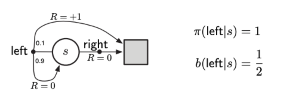
The estimates of ordinary importance sampling will typically have infinite variance, and thus unsatisfactory convergence properties, whenever the scaled returns have infinite variance—and this can easily happen in o↵-policy learning when trajectories contain loops. A simple example is shown inset in implementation below. There is only one nonterminal state $s$ and two actions, right and left. The right action causes a deterministic transition to termination, whereas the left action transitions, with probability 0.9, back to $s$ or, with probability 0.1, on to termination. The rewards are $+1$ on the latter transition and otherwise zero. Consider the target policy that always selects left. All episodes under this policy consist of some number (possibly zero) of transitions back to $s$ followed by termination with a reward and return of +1. Thus the value of s under the target policy is 1 ($\gamma$ = 1). Suppose we are estimating this value from o↵-policy data using the behavior policy that selects right and left with equal probability.

ACTION_BACK = 0
ACTION_END = 1

# behavior policy
def behavior_policy():
    return np.random.binomial(1, 0.5)

# target policy
def target_policy():
    return ACTION_BACK

# one turn
def play():
    # track the action for importance ratio
    trajectory = []
    while True:
        action = behavior_policy()
        trajectory.append(action)
        if action == ACTION_END:
            return 0, trajectory
        if np.random.binomial(1, 0.9) == 0:
            return 1, trajectory

def figure_5_4():
    runs = 10
    episodes = 1000000
    for run in range(runs):
        rewards = []
        for episode in range(0, episodes):
            reward, trajectory = play()
            if trajectory[-1] == ACTION_END:
                rho = 0
            else:
                rho = 1.0 / pow(0.5, len(trajectory))
            rewards.append(rho * reward)
        rewards = np.add.accumulate(rewards)
        estimations = np.asarray(rewards) / np.arange(1, episodes + 1)
        plt.plot(estimations)
    plt.ylim(-.1, 3)
    plt.xlabel('Episodes (log scale)')
    plt.ylabel('Ordinary Importance Sampling')
    plt.xscale('log')
    plt.plot()

figure_5_4()

This implemented figure shows ten independent runs of the first-visit MC algorithm using ordinary importance sampling. Even after millions of episodes, the estimates fail to converge to the correct value of 1. In contrast, the weighted importance-sampling algorithm would give an estimate of exactly 1 forever after the first episode that ended with the left action.

$\begin{aligned} Var[V] &= \mathbb{E}[V -\bar{V}]^2 = \mathbb{E}[V^2] - \bar{V}^2 \text{ (note }\bar{V}\text{ is finite)}\\ &=\mathbb{E}_{b}\left[\left(\prod_{t=0}^{T-1} \frac{\pi\left(A_{t} \mid S_{t}\right)}{b\left(A_{t} \mid S_{t}\right)} G_{0}\right)^{2}\right] \\&= \frac{1}{2} \cdot 0.1\left(\frac{1}{0.5}\right)^{2} \\ &+\frac{1}{2} \cdot 0.9 \cdot \frac{1}{2} \cdot 0.1\left(\frac{1}{0.5} \frac{1}{0.5}\right)^{2} \\ &+\frac{1}{2} \cdot 0.9 \cdot \frac{1}{2} \cdot 0.9 \cdot \frac{1}{2} \cdot 0.1\left(\frac{1}{0.5} \frac{1}{0.5} \frac{1}{0.5}\right)^{2} \\ &+\cdots -\bar{V}^2\\&= 0.1 \sum_{k=0}^{\infty} 0.9^{k} \cdot 2^{k} \cdot 2-\bar{V}^2=0.2 \sum_{k=0}^{\infty} 1.8^{k} - \bar{V}^2\\&=\infty \end{aligned}$

And this proves why it is unstable and has large varaiance of V.

Incremental Implementation

For saving memory and decreasing computational time, we can calculate the increment, introduced in chapter 2.

Denote $\rho_{t:T(t)-1}$ as $W_k$, then we have $\displaystyle V_{n}=\frac{\sum_{k=1}^{n-1} W_{k} G_{k}}{\sum_{k=1}^{n-1} W_{k}},$ and let $C_{n}=\sum_{k=1}^{n} W_{k}$, then,

$\begin{aligned} V_{n+1} &=\frac{\sum_{k=1}^{n-1} W_{k} G_{k}+W_{n} G_{n}}{\sum_{k=1}^{n} W_{k}} \\ &=\frac{\sum_{k=1}^{n-1} W_{k} \frac{\sum_{k=1}^{n-1} W_{k} G_{k}}{\sum_{k=1}^{n-1} W_{k}}+W_{n} G_{n}}{\sum_{k=1}^{n} W_{k}} \\ &=\frac{C_{n-1} V_{n}+W_{n} G_{n}}{C_{n}} \\ &=\frac{\left(C_{n}-W_{n}\right) V_{n}+W_{n} G_{n}}{C_{n}} \\ &=V_{n}+\frac{W_{n}}{C_{n}}\left[G_{n}-V_{n}\right] \end{aligned}$

And therefore we could get the update rule:

$V_{n+1}=V_{n}+\frac{W_{n}}{C_{n}}\left[G_{n}-V_{n}\right]$

$C_{n+1}=C_{n}+W_{n+1},\left(C_{0}=0\right)$

The algorithm for off-policy MC prediction using increment update rule is shown below.

When $W = 0 \Rightarrow \pi(A_t|S_t) = 0 \Rightarrow$ behavior policy $b$ produces a new action not within $\pi$, the episode will be terminated.

Off-policy Monte Carlo Control

After prior intruduction, we can have the off-policy MC control algorithm, based on GPI and weighted importance sampling, for estimating $\pi_*$ and $q_*$. The target policy $\pi \approx \pi_*$ is the greedy policy with respect to $Q$, which is an estimate of $q_*$. The behavior policy $b$ can be anything, but in order to assure convergence of $\pi$ to the optimal policy, an infinite number of returns must be obtained for each pair of state and action. This can be assured by choosing $b$ to be "$\epsilon$-soft.

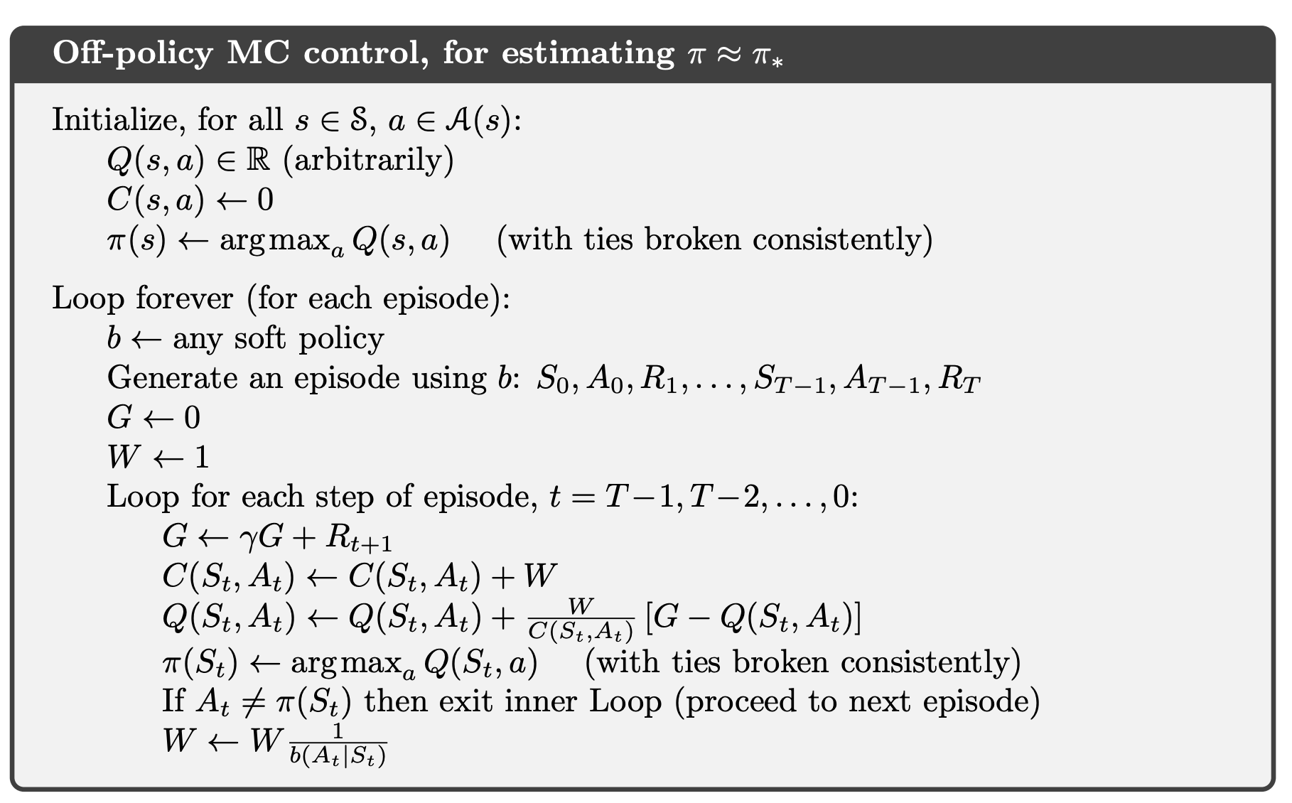
$\pi$ is deterministic instead of soft, and $b$ is soft to make sure the exploration of actions and deterministic of $\pi$. It is also worth noting that in the algorithm box above, $\displaystyle W \leftarrow W \frac{\pi\left(A_{t} \mid S_{t}\right)}{b\left(A_{t} \mid S_{t}\right)} = \frac{1}{b\left(A_{t} \mid S_{t}\right)}$ as the target policy in deterministic $\Rightarrow \pi(A_t | S_t) =1$

Several optional importance sampling methods to approximate value function are introduced in the book, but will not be verified here.